is_president(barack_obama)
We have shown how knowledge can be represented in first-order logic, and how rule-based expert systems expressed in logic can be constructed and used. We now look at how to take some known facts about a domain and deduce new facts from them. This will, in turn, enable agents to prove things, i.e., to start with a set of statements we believe to be true (axioms) and deduce whether another statement (theorem) is true or not. We will first look at how to tell whether a sentence in propositional logic is true or false. This will suggest some equivalences between propositional sentences, which allow us to rewrite sentences to other sentences which mean the same thing, regardless of the truth or meaning of the individual propositions they contains. These are reversible inferences, in that deduction can be applied either way. We then look at propositional and first-order inference rules in general, which enable us deduce new sentences if we know that certain things are true, and which may not be reversible.
In propositional logic — where we are restricted to expressing sentences where propositions are true or false — we can check whether a particular statement is true or false by working out the truth of ever larger substatements using the truth of the propositions themselves. To work out the truth of substatements, we need to know how to deal with truth assignments in the presence of connectives. For instance, if we know that is_president(barack_obama) and is_male(barack_obama) are true, then we know that the sentence:
is_male(barack_obama)
is_president(barack_obama)
is also true, because we know that a sentence of the form P Q is
true when P is true and Q is true.
The truth values of connectives given the truth values of the propositions they contain is presented in the following truth table:
| P | Q | ¬P | P Q |
P  Q |
P  Q |
P  Q |
|
| True | True | False | True | True | True | True | |
| True | False | False | False | True | False | False | |
| False | True | True | False | True | True | False | |
| False | False | True | False | False | True | True |
This table allows us to read the truth of the connectives in the following manner. Suppose we are looking at row three. This says that, if P is false and Q is true, then
Q is false Q is true Q is true Q is false Note that, if P is false, then regardless of whether
Q is true or false, the statement P Q is
true. This takes a little getting used to, but can be a very useful
tool in theorem proving: if we know that something is false, it can
imply anything we want it to! So, the following sentence is true:
"Barack Obama is female" implies that "Barack Obama is an alien",
because the premise that Barack Obama is female was false, so
the conclusion that Barack Obama is an alien can be deduced in
a sound way.
Each row of a truth table defines the connectives for a particular assignment of true and false to the individual propositions in a sentence. We call each assignment a model: it represents a particular possible state of the world. For two propositions P and Q there are four models.
For propositional sentences in general, a model is also just a particular assignment of truth values to its individual propositions. A sentence with n propositions will have 2n possible models, and so 2n rows in its truth table. A sentence S will be true or false for a given model M — when S is true we say 'M is a model of S'.
Sentences which are always true, regardless of the truth of the individual propositions, are called tautologies (or valid sentences). Tautologies are true for all models. For instance, if I said that "Tony Blair is prime minister or Tony Blair is not prime minister", this is largely a content-free sentence, because we could have replaced the predicate of being Tony Blair with any predicate and the sentence would still have been correct.
Tautologies are not always as easy to notice as the one above, and we can use truth tables to be certain that a statement we have written is true, regardless of the truth of the individual propositions it contains. To do this, the columns of our truth table will be headed with ever larger sections of the sentence, until the final column contains the entire sentence. As before, the rows of the truth table will represent all the possible models for the sentence, i.e. each possible assignment of truth values to the individual propositions in the sentence. We will use these initial truth values to assign truth values to the subsentences in the truth table, then use these new truth values to assign truth values to larger subsentences and so on. If the final column (the entire sentence) is always assigned true, then this means that, whatever the truth values of the propositions being discussed, the entire sentence will turn out to be true.
For example, the following is a tautology:
S: (X
(Y Z))
((X Y)
(X
Z))
In English, sentence, S says that X implies Y and Z if and only if X implies Y and X implies Z. The truth table for this sentence will look like this:
| X | Y | Z | Y Z
| X Y
| X Z
| X (YZ)
| ((X Y)(XZ))
| S |
| true | true | true | true | true | true | true | true | true | true | true | false | false | true | false | false | false | true | true | false | true | false | false | true | false | false | true | true | false | false | false | false | false | false | false | true | false | true | true | true | true | true | true | true | true | false | true | false | false | true | true | true | true | true | false | false | true | false | true | true | true | true | true | false | false | false | false | true | true | true | true | true |
We see that that the seventh and eighth columns
— the truth values which have been built up from the previous
columns — have exactly the same truth values in each row. Because
our sentence is made up of the two subsentences in these columns, this
means that our overall equivalence must be correct. The truth of this
statement demonstrates that the connectives and
are related by a property called distributivity, which we come
back to later on.
Truth tables give us our first (albeit simple) method for proving a theorem: check whether it can be written in propositional logic and, if so, if it is a tautology, then it must be true. So, for instance, if we were asked to prove this theorem from number theory:
 n, m
((sigma(n) = n tau(n) = m)
(tau(n) = m
sigma(n) =\= n))
then we could prove it straight away, because we know that this is a tautology:
(XY)
(Y
¬X)
As we know this is a tautology, and that our number theory theorem fits into the tautology (let X represent the proposition sigma(n)=n, and so on), we know that the theorem must be true, regardless of what tau and sigma mean. (As an exercise, show that this is indeed a tautology, using a truth table).
As well as allowing us to prove trivial theorems,
tautologies enable us to establish that certain sentences are
saying the same thing. In particular, if we can show that
A B is a tautology then we know
A and B are true for exactly the same models, i.e. they
will have identical columns in a truth table. We say that A and
B are logically equivalent, written as the
equivalence A  B.
(Clearly and mean the same thing here, so why use two different
symbols? It's a technical difference: A B is a sentence of propositional logic,
whereas A B is a claim we make
outside the logic.)
In natural language, we could replace the phrase "There's only one Tony Blair" by "Tony Blair is unique", in sentences, because basically the phrases mean the same thing. We can do exactly the same in logical languages, with an advantage: because we are being more formal, we will have mathematically proved that two sentences are equivalent. This means that there is absolutely no situation in which one sentence would be interpreted in a different way to another, which is certainly possible with natural language sentences about Tony Blair.
Equivalences allow us to change one sentence into
another without affecting the meaning, because we know that replacing
one side of an equivalence with the other will have no effect whatsoever
on the semantics: it will still be true for the same models. Suppose we
have a sentence S with a subexpression A, which we write as S[A]. If we
know A B then we can be sure the semantics
of S is unaffected if we replace A with B, i.e. S[A] S[B].
Moreover, we can also use A B to replace
any subexpression of S which is an instance of A. An instance of a
propositional expression A is a 'copy' of A where some of the
propositions of have been consistently replaced by new subexpressions, e.g.
every P has been replaced by ¬Q. We call
this replacement a substitution, a mapping from propositions to
expressions. Applying a substitution U to a sentence S, we get a new
sentence S.U which is an instance of S. It is easy to show that if A
B then A.U B.U
for any substitution U, i.e. an instance of an equivalence is also an
equivalence. Hence an equivalence A B
allows us to change a sentence S[A'] to a logically equivalent
one S[B'] if we have substitution U such that A' = A.U and B' = B.U.
The power to replace subexpressions allows use to prove theorems with
equivalences: in the above example, given a theorem S[A'] S[B'] we can use the equivalence A B to rewrite the theorem to the equivalent
S[A'] S[A'], which we know to be true.
Given a set of equivalences we can prove (or disprove) a complex theorem
by rewriting it to something logically equivalent that we already know
to be true (or false).
The fact that we can rewrite instances of A to instances of B is expressed in the rewrite rule A => B. Of course, we can also rewrite Bs to As, so we could use the rewrite rule B => A instead. However, it's easy to see that having an agent use both rules is dangerous, as it could get stuck in a loop A => B => A => B => ... and so on. Hence, we typically use just one of the rewrite rules for a particular equivalence (we 'orient' the rule in a single direction). If we do use both then we need to make sure we don't get stuck in a loop.
Apart from proving theorems directly, the other main use for rewrite rules is to prepare a statement for use before we search for the proof, as described in the next lecture. This is because some automated deduction techniques require a statement to be in a particular format, and in these cases, we can use a set of rewrite rules to convert the sentence we want to prove into a logically equivalent one which is in the correct format.
Below are some common equivalences which automated theorem provers can use as rewrite rules. Remember that the rules can be read both ways, but that in practice either i) only one direction is used or ii) a loop-check is employed. Note also that these are true of sentences in propositional logic, so they can also be used for rewriting sentences in first-order logic, which is just an extension of propositional logic.
You will be aware of the fact that some arithmetic operators have a property that it doesn't matter which way around you give the operator input. We call this property commutativity. For example, when adding two numbers, it doesn't matter which one comes first, because a+b = b+a for all a and b. The same is true for multiplication, but not true for subtraction and division.
The , and connectives (which operate on two
subsentences), also have the commutativity property. We can express
this with three tautologies:
P Q
 Q P
P Q
Q P
P Q
Q P
So, if it helps to do so, whenever we see P Q, we can rewrite it as Q P, and similarly for the other two
commutative connectives.
Brackets are useful in order to tell us when to perform calculations in arithmetic and when to evaluate the truth of sentences in logic. Suppose we want to add 10, 5 and 7. We could do this: (10 + 5) + 7 = 22. Alternatively, we could do this: 10 + (5 + 7) = 22. In this case, we can alter the bracketing and the answer still comes out the same. We say that addition is associative because it has this property with respect to bracketing.
The and connectives are associative. This makes
sense, because the order in which we check truth values doesn't matter
when we are working with sentences only involving or only involving . For instance, suppose we wanted to
know the truth of P (Q R). To do this, we just need to
check that every proposition is true, in which case the whole sentence
will be true, otherwise the whole sentence will be false. So, it
doesn't matter how the brackets are arranged, and hence the is associative.
Similarly, suppose we wanted to work out the truth of:
(P
Q)
(R
(X Z))
Then all we need to do is check whether one of these propositions is true, and the bracketing is immaterial. As equivalences, then, the two associativity results are:
(P Q) R
P (Q R)
(P Q) R
P (Q R)
Our last analogy with arithmetic will involve a well-used technique for playing around with algebraic properties. Suppose we wanted to work out: 10 * (3 + 5). We could do it like this: 10 * (3 + 5) = 10 * 8 = 80. Or we could do it like this: (10 * 3) + (10 * 5) = 30 + 50 = 80. In general, we know that, for any numbers, a, b and c: a * (b + c) = (a * b) + (a * c). In this case, we say that multiplication is distributive over addition.
You guessed it, we can distribute some of the connectives too. In
particular, is distributive over
and vice versa: is also distributive over . We can present these as equivalences
as follows:
P (Q R)
(P Q) (P R)
P (Q R)
(P Q) (P R)
Also, we saw earlier that is
distributive over , and the same
is true for over . Therefore:
P (Q R)
(P Q) (P R)
P (Q R)
(P Q) (P R)
Parents are always correcting their children for the
use of double negatives, but we have to be very careful with them in
natural language: "He didn't tell me not to do it" doesn't necessarily
mean the same as "He did tell me to do it". The same is true with
logical sentences: we cannot, for example, change ¬(P Q) to (¬ P ¬Q) without risking the meaning of
the sentence changing. However, there are certain cases when we can
alter expressions with negation. Two possibilities are given by de
Morgan's law below, and we can also simplify statements by removing
double negation. These are cases when a proposition has two negation
signs in front of it, like this: ¬¬P.
You may be wondering why on earth anyone would ever write down a sentence with such a double negation in the first place. Of course, you're right. As humans, we wouldn't write a sentence in logic like that. However, remember that our agent will be doing search using rewrite rules. It may be that as part of the search, they introduce a double negation, by following a particular rewrite rule to the letter. In this case, the agent would probably tidy it up by using this equivalence:
¬¬P P
Continuing with the relationship between and , we can also use De Morgan's Law to
rearrange sentences involving negation in conjunction with these
connectives. In fact, there are two equivalences which, taken as a
pair are called De Morgan's Law:
¬ (P Q)
¬P
¬Q
¬ (P Q)
¬P
¬Q
These are important rules and it is worth spending some time thinking about why they are true.
The contraposition equivalence is as follows:
P Q
¬Q ¬P
This may seem a little strange at first, because it appears that we have said nothing in the first sentence about ¬Q, so how can we infer anything from it in the second sentence? However, suppose we know that P implies Q, and we saw that Q was false. In this case, if we were to imply that P was true, then, because we know that P implies Q, we also know that Q is true. But Q was false! Hence we cannot possibly imply that P is true, which means that we must imply that P is false (because we are in propositional logic, so P must be either true or false). This argument shows that we can replace the first sentence by the second one, and it is left as an exercise to construct a similar argument for the vice-versa part of this equivalence.
The following miscellaneous equivalence rules are often useful during rewriting sessions. The first two allow us to completely get rid of implication and equivalence connectives from our sentences if we want to:
Q
¬P Q
(this one is very useful)
Q
(P
Q ) (Q P)
The next two allow truth values to be determined regardless of the truth of the propositions.
¬ P
False
¬ P
True
Here the "False" symbol stands for the proposition which is always false: no matter what truth values you give to other propositions in the sentence, this one will always be false. Similarly, the "True" symbol stands for the proposition which is always true. In first-order logic we can treat them as special predicates with the same properties.
Equivalence rules can be used to show that a complicated looking sentence is actually just a simple one in disguise. For this example, we shall show that this sentence:
(A B)
( ¬ A B)
conveys a meaning which is actually much simpler than you would think on first inspection.
We can simplify this, using the following chain of rewrite steps based on the equivalences we've stated above:
B)
(¬A ¬¬B)
¬ Q =>
¬(P Q)
B)
¬ (A ¬B)
:
P Q => Q P
B)
¬ (¬ B A)
Q => P Q
B)
¬ (B A)
Q => (P Q)
(Q P)
B)
(B A))
¬ (B A)
:
(P Q) R =>
P (Q R)
B)
((B A)
¬ (B A))
¬P => False
B)
False
:
So, what does this mean? It means that our original sentence was always false: there are no models which would make this sentence true. Another way to think about this is that the original sentence was inconsistent with the rules of propositional logic. In general, proving theorems by proving that they're negation rewrites to False is an example of proof by contradiction, which we discuss below.
Note that the first step of this simplification
routine was to insert a double negation! Also, at some stages, the
rewritten sentence looked more complicated than the original, so we
seemed to be making matters worse, which is quite common. Is there any
other way to simplify the original statement? Of course, you'll still
end up with the answer false, but there might be a quicker way to get
there. You may get the feeling you are solving a search problem, which,
of course, is exactly what you're doing. If you think about this
sentence, it may become obvious why it is false: for (¬P Q) to be true, P must be false and Q must be
true. But then what about the conjoined equivalence?
|
|
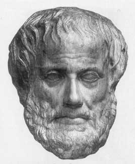
Aristotle was a Greek Philosopher and Mathematician who is often regarded as the father of logic. Several of Aristotle's treatises were grouped together under the title Organon ("Instrument") which comprised his works on logic. Amongst other things, he introduced Syllogisms, which encapsulated rules of inference such as Modus Ponens described below. Read a biography of Aristotle here. |
Equivalence rules are particularly useful because of the vice-versa aspect, which means that we can search backwards and forwards in a search space using them. Hence, we can perform bi-directional search, which is a bonus. However, what if we know that one sentence (or set of sentences) being true implies that another set of sentences is true. For instance, the following sentence is used ad nauseum in logic text books:
All men are mortal
Socrates was a man
Hence, Socrates is mortal
This is an example of the application of a rule of deduction known as Modus Ponens. We see that we have deduced the fact that Socrates is mortal from the two true facts that all men are mortal and Socrates was a man. So, because we know that the rule about men being mortal and the classification of Socrates as a man are true, we can infer with certainty (because we know that modus ponens is sound), that Socrates is going to die - which, of course, he did. Of course, it doesn't make sense to go backwards as with equivalences: we would deduce that, Socrates being mortal implies that he was a man and that all men are mortal!
The general format for the modus ponens rule is as follows: if we have a true sentence which states that proposition A implies proposition B and we know that proposition A is true, then we can infer that proposition B is true. The notation we use for this is as follows:
|
A B, A
|
|
| B |
This is an example of an inference rule. The comma above the line indicates we know both these things in our knowledge base, and the line stands for the deductive step. That is, if we know that both the propositions above the line are true, then we can deduce that the proposition below the line is also true. In general, an inference rule
| A |
|
| B |
is sound if we can be sure that A entails B, i.e. B is
true when A is true. More formally, A entails B means that if M is a
model of A then M is also a model of B. We write this as A  B.
This gives us a way to check the soundness of propositional inference rules: (i) draw up a logic table for both A and B evaluating them for all models and (ii) check that whenever A is true, then B is also true. We don't care here about the models for which A is false.
For instance, the truth table for the modus ponens rule is really the same as the one for the implication connective. It looks like this:
| A | B | AB |
| True | True | True |
| True | False | False |
| False | True | True |
| False | False | True |
This is a trivial example, but it highlights how we use truth tables:
the first line is the only one where both above-line propositions (A and
A B) are true. We see that on this
line, the proposition B is also true. This shows us that we have an
entailment: the above-line propositions entail the below-line one.
To see why such inference rules are useful, remember what the main application of automated deduction is: to prove theorems. Theorems are normally part of a larger theory, and that theory has axioms. Axioms are special theorems which are taken to be true without question. Hence whenever we have a theorem statement we want to prove, we should be able to start from the axioms and deduce the theorem statement using sound inference rules such as modus ponens.
Below are some more propositional inference rules:
In English, this says that "if you know that lots of things are all
true, then you know that any one of them is also true". It means that
you can simplify a conjunction by just taking one of the conjuncts (in
effect, eliminating the s).
|
A1
A2
...
An
|
|
| Ai |
Note that 1 ≤ i ≤ n.
In English, this says that "if we know that a lot of things are true, then we know that the conjunction of all of them is true", so we can introduce conjunction ('and') symbols.
| A1, A2, ..., An |
|
|
A1
A2
...
An
|
This may not seem to be saying much. However, imagine that we are working with a lot of different sentences at different places in our knowledge base, and we know some of them are true. Then we can make a larger sentence out of them by conjoining the smaller ones.
If we know that one thing is true, then we know that a sentence where that thing is in a disjunction is true. For example, we know that "Tony Blair is prime minister" is true. From this, we can infer any disjunction as long as we include this true sentence as a disjunct. So, we can infer that "Tony Blair is prime minister or the moon is made of blue cheese", which makes perfect sense.
| Ai |
|
|
A1
A2
...
An
|
Again, 1 ≤ i ≤ n.
Suppose that we knew the sentence "Tony Blair is prime minister or the moon is made of blue cheese", is true, and we later found out that the moon isn't in fact made of cheese. Then, because the first (disjoined) sentence is true, we can infer that Tony Blair is indeed prime minister. This typifies the essence of the unit resolution rule:
|
(A B), ¬ B
|
|
| A |
The generalised version of this inference rule is the subject of a whole area of Artificial Intelligence research known as resolution theorem proving, which we cover in detail in the next lecture.
We proposed first-order logic as a good knowledge representation language rather than propositional logic because it is more expressive, so we can write more of our sentences in logic. So the sentences we are going to want to apply rewrites and inference rules will include quantification. All of the rewrite rules we've seen so far can be used in propositional logic (and hence first-order logic). We now consider rules in which rely on information about the quantifiers, so are not available to an agent working with a propositional logic representation scheme.
Before we look at first-order inference rules we need to pause to consider what it means for such an inference rule to be sound. Earlier we defined this as meaning the top entails the bottom: that any model of the former was a model of the latter. But first-order logic introduces new syntactic elements (constants, functions, variables, predicates and quantifiers) alongside the propositional connectives. This means we need to completely revise our definition of model, a notion of a 'possible world' which defines whether a sentence is true or false in that world.
A propositional model was just an assignement of truth values to propositions. In contrast, a first-order model is a pair (Δ, Θ) where
First-order logic allows us to talks about properties of objects, so the first job for our model (Δ, Θ) is to assign a meaning to the terms which represent objects. A ground term is any combination of constant and function symbols, and Θ maps each individual ground term to a specific object in Δ. This means that a ground term refers to a single specific object. The meaning of subterms is always independent of the term they appear in.
The particular way that terms are mapped to objects depends on the model. Different models can define terms as refering to different things. Note that although father(john) and jack are separate terms, they might both be mapped to the same object (say Jack) in Δ. That is, the two terms are syntactically different but (in this model) they are semantically the same, i.e. they both refer to the same thing!
Terms can also contain variables (e.g. father(X)) — these are non-ground terms. They don't refer to any specific object, and so our model can't assign any single meaning to them directly. We'll come back to what variables mean.
Predicates take a number of arguments (which for now we assume are ground terms) and represent a relationship between those arguments which can be true or false. The semantics of an n-ary predicate p(t1,...tn) are defined by a model (Δ, Θ) as follows: we first calculate the n objects that the arguments refer to Θ(t1), ..., Θ(tn). Θ maps p to a function P: Δn→{true,false} which defines whether p is true for those n elements of Δ. Different models can assign different functions P, i.e. they can provide different meanings for each predicate.
Combining predicates, ground terms and propositional connectives gives us ground formulae, which don't contain any variables. They are definite statements about specific objects.
So what do sentences containing variables mean? In other words, how does a first-order model decide whether such a sentence is true or false? The first step is to ensure that the sentence does not contain any free variables, variables which are not bound by (associated with) a quantifier. Strictly speaking, a first-order expression is not a sentence unless all the variables are bound. However, we usually assume that if a variable is not explicitly bound then really it is implicitly universally quantified.
Next we look for the outermost quantifier in our sentence. If this
is X then we consider the truth of the
sentence for every value X could take. When the outermost
quantifier is  X we need to find just a
single possible value of X. To make this more formal we can
use a concept of substitution. Here {X\t} is a substitution
which replaces all occurances of variable X with a term representing an object t:
X. A is true if and only if A.{X\t}
for all t in Δ
X. A is true if and only if A.{X\t} for
at least one t in Δ
Repeating this for all the quantifiers we get a set of ground formulae which we have to check to see if the original sentence is true or false. Unfortunately, we haven't specificed that our domain Δ is finite — for example, it may contain the natural numbers — so there may be a infinite number of sentences to check for a given model! There may be also be an infinite number of models..So although we have a proper definition of model, and hence a proper semantics for first-order logic, so we can't rely on having a finite number of models as we did when drawing propositional truth tables.
Now we have a clear definition of a first-order model is, we can define soundness for first-order inference rules in the same way as we did for propositional inference rules: the rule is sound if given a model of the sentences above the line, this is always a model of the sentence below.
To be able to specify these new rules, we must use the notion of substitution. We've already seen substitutions which replace propositions with propositional expressions (7.2 above) and other substitutions which replace variables with terms that represent a given object (7.5 above). In this section we use substitutions which replace variables with ground terms (terms without variables) — so to be clear we will call these ground substitutions. Another name for a ground substitution is an instantiation,
For example, if we start with the wonderfully optimistic sentence that
everyone likes everyone else: X, Y
(likes(X, Y)), then we can choose particular values for X and Y. So,
we can instantiate this sentence to say: likes(george, tony). Because
we have chosen a particular value, the quantification no longer makes
sense, so we must drop it.
The act of performing an instantiation is a function, as there is only one possible outcome, so we can write it as a function. The notation
Subst({X/george, Y/tony}, likes(X,Y)) = likes(george, tony)
indicates that we have made a ground substitution.
We also have to recognise that we are working with sentences which form part of a knowledge base of many such sentences. More to the point, there will be constants which appear throughout the knowledge base, and some which are local to a particular sentence.
For any sentence, A, containing a universally quantified variable, v, then for any ground term, g, we can substitute g for v in A. We write the following to represent this rule:
|
v A
|
|
| Subst({v/g}, A) |
As an example (from Russell and Norvig), this rule can be used on the
following sentence: X, likes(X,
ice_cream) to substitute the variable 'ben' for X, giving us the
sentence likes(ben, ice_cream). In English, this says that, given that
everyone likes ice cream, we can infer that Ben likes ice cream. This
is not exactly rocket science, and it is worth bearing in mind that,
beneath all the fancy symbols in logic, we're really only saying
simple things.
For a sentence, A, with an existentially quantified variable, v, then, for every constant symbol k, that does not appear anywhere else in the knowledge base, we can substitute k for v in A:
|
v A
|
|
| Subst({v/k}, A) |
For an example, if we know that X (likes(X,ice_cream)), then we can
choose a particular name for X. We could choose ben for this, giving
us: likes(ben, ice_cream), but only if the constant ben does not
appear anywhere else in our knowledge base.
So, why the condition about the existential variable being unique to the new sentence? Basically, what you are doing here is giving a particular name to a variable you know must exist. It would be unwise to give this a name which already exists. For example, suppose we have the predicates brother(john,X), sister(john, susan) then, when instantiating X, it would be unwise to choose the term susan for the constant to ground X with, because this would probably be a false inference. Of course, it's not impossible that John would have a sister named Susan and also a brother named Susan, but it is not likely. However, if we choose a totally new constant, then there can be no problems and the inference is guaranteed to be correct.
For any sentence, A, and variable, v, which does not occur in A, then for any ground term, g, that occurs in A, we can turn A into an existentially quantified sentence by substituting v for g:
| A |
|
|
v
Subst({g/v}, A)
|
So, for example, if we know that likes(jerry, ice_cream), then we can
infer that X (likes(X,
ice_cream)), because the constant jerry does not appear anywhere else
in the original sentence. The conditions that v and g do not occur in
A is for similar reasons as those given for the previous rule. As an
exercise, find a situation where ignoring this condition would mean
that the inferred sentence did not follow logically from the premise
sentence.
We look now at how to get an agent to prove a given theorem using various search strategies. We have noted in previous lectures that, to specify a search problem, we need to describe the representation language for the artefacts being searched for, the initial state, the goal state (or some information about what a goal should look like), and the operators: how to go from one state to another.
We can state the problem of proving a given theorem from some axioms as a search problem. Three different specifications give rise to three different ways to solve the problem, namely forward and backward chaining and proof by contradiction. In all of these specifications, the representation language is predicate logic (not surprisingly), and the operators are the rules of inference, which allow us to rewrite a set of sentences as another set. We can think of each state in our search space as a sentence in first order logic. The operators will traverse this space, finding new sentences. However, we are really only interested in finding a path from the start states to the goal state, as this path will constitute a proof. (Note that there are other ways to prove theorems such as exhausting the search for a counterexample and finding none - in this case we don't have a deductive proof for the truth of the theorem, but we know it is true).
Only the initial state of the space and the details of the goal differ in the three following approaches.
Suppose we have a set of axioms which we know are true statements about the world. If we set these to each be an initial state of the search space, and we set the goal state to be our theorem statement, then this is a simple approach which can be used to prove theorems. We call this approach forward chaining, because the agent employing the search constructs chains of reasoning, from the axioms, hopefully to the goal. Once a path has been found from the axioms to the theorem, this path constitutes a proof and the problem has been solved.
However, the problem with forward chaining in general is that it cannot easily use the goal (theorem statement) to drive the search. Hence it really must just explore the search space until it comes across the solution. Goal-directed searches are often more effective than non-goal directed ones like forward chaining.
Given that we are only interested in constructing the path, we can set our initial state to be the theorem statement and search backwards until we find an axiom (or set of axioms). If we restrict ourselves to just using equivalences as rewrite rules, then this approach is OK, because we can use equivalences both ways, and any path from the theorem to axioms which is found will provide a proof. However, if we use inference rules to traverse from theorem to axioms, then we will have proved that, if the theorem is true, then the axioms are true. But we already know that the axioms are true! To get around this, we must invert our inference rules and try to work backwards. That is, the operators in the search basically answer the question: what could be true in order to infer the state (logical sentence) we are at right now? If our agent starts searching from the theorem statement and reaches the axioms, it has proved the theorem. This is also problematic, because there are numerous answers to the inversion question, and the search space gets very large.
So, forward chaining and backward chaining both have drawbacks. Another approach is to think about proving theorems by contradiction. These are very common in mathematics: mathematicians specify some axioms, then make an assumption. After some complicated mathematics, they have shown that an axiom is false (or something derived from the axioms which did not involve the assumption is false). As the axioms are irrefutably correct, this means that the assumption they made must be false. That is, the assumption is inconsistent with the axioms of the theory. To use this for a particular theorem which they want to prove is true, they negate the theorem statement and use this as the assumption they are going to show is false. As the negated theorem must be false, their original theorem must be true. Bingo!
We can program our reasoning agents to do just the same. To specify this as a search problem, therefore, we have to say that the axioms of our theory and the negation of the theorem we want to prove are the initial search states. Remembering our example in section 7.2, to do this, we need to derive the False statement to show inconsistency, so the False statement becomes our goal. Hence, if we can deduce the false statement from our axioms, the theorem we were trying to prove will indeed have been proven. This means that, not only can we use all our rules of inference, we also have a goal to aim for.
As an example, below is the input to the Otter theorem prover for the trivial theorem about Socrates being mortal. Otter searches for contradictions using resolution, hence we note that the theorem statement - that Socrates is mortal - is negated using the minus sign. We discuss Otter and resolution theorem proving in the next two lectures.
Input:
set(auto).
formula_list(usable).
all x (man(x)->mortal(x)). % For all x, if x is a man then x is mortal
man(socrates).             % Socrates is a man
-mortal(socrates).         % Socrates is immortal (note: negated)
end_of_list.
Otter has no problem whatsoever proving this theorem, and here is the output:
Output:
---------------- PROOF ----------------

1 [] -man(x)|mortal(x).
2 [] -mortal(socrates).
3 [] man(socrates).
4 [hyper,3,1] mortal(socrates).
5 [binary,4.1,2.1] $F.

------------ end of proof -------------